Table of Contents
Probability is the maths of uncertainty: how likely something is to happen. It shows up in weather forecasts, games, medical tests, sport, insurance and machine learning. It is also the area of maths where intuition goes wrong most often, which is exactly what makes it fun to learn.
This guide starts from the basic definition and builds up through the rules you need, with each idea tested by a short Python simulation. Computers can repeat an experiment hundreds of thousands of times in a second, so you can check a calculation against reality instead of just trusting it. Every number below comes from running the code.
What is probability?
When all outcomes are equally likely, the probability of an event is:
The basic formula
probability = number of outcomes you want ÷ total number of possible outcomes, when every outcome is equally likely.
A fair die has 6 equally likely outcomes, so the probability of rolling a 4 is 1/6. Probabilities are always between 0 (impossible) and 1 (certain), and can be written as fractions, decimals or percentages: 1/6, about 0.167, or about 16.7%. If fractions still feel shaky, our guide on understanding fractions is a good warm-up, and percentages covers converting between them.
Counting outcomes: two dice
Roll two dice and add them. Which total is most likely? Many people guess every total is equally likely, but they are not. There are 6 × 6 = 36 equally likely outcomes (a 1 and a 2 is different from a 2 and a 1), and more of them add up to 7 than to anything else. Here is the exact count next to a simulation of 100,000 rolls:
import random
from collections import Counter
from fractions import Fraction

# Exact: count the 36 equally likely outcomes of two dice
exact = Counter(a + b for a in range(1, 7) for b in range(1, 7))

# Simulated: roll two dice 100,000 times
random.seed(7)
rolls = 100_000
sim = Counter(random.randint(1, 6) + random.randint(1, 6) for _ in range(rolls))

print("sum  ways  exact   simulated")
for total in range(2, 13):
    p = Fraction(exact[total], 36)
print(f"{total:>3} {exact[total]:>4} {float(p):.3f} {sim[total] / rolls:.3f}")sum ways exact simulated
2 1 0.028 0.028
3 2 0.056 0.056
4 3 0.083 0.085
5 4 0.111 0.110
6 5 0.139 0.138
7 6 0.167 0.168
8 5 0.139 0.139
9 4 0.111 0.113
10 3 0.083 0.083
11 2 0.056 0.054
12 1 0.028 0.027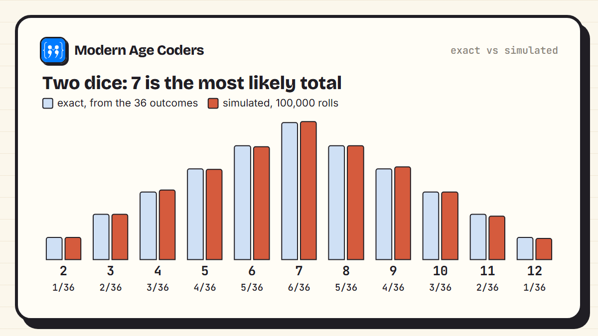
A total of 7 can be made 6 ways (1+6, 2+5, 3+4, 4+3, 5+2, 6+1), so its probability is 6/36, about 0.167. A total of 2 needs a double 1, just one way. The simulation agreed with the counting to within a few thousandths for every total. This is why 7 matters so much in many board games.
The law of large numbers
A fair coin lands heads with probability 1/2. That does not mean 10 flips give exactly 5 heads. It means that over many flips, the proportion of heads gets closer and closer to 0.5:
import random

random.seed(3)
heads = 0
checkpoints = {10, 100, 1_000, 10_000, 100_000, 1_000_000}
for flip in range(1, 1_000_001):
    heads += random.random() < 0.5
    if flip in checkpoints:
print(f"{flip:>9,} flips: {heads / flip:.4f} heads")10 flips: 0.6000 heads
100 flips: 0.4300 heads
1,000 flips: 0.5090 heads
10,000 flips: 0.5054 heads
100,000 flips: 0.5019 heads
1,000,000 flips: 0.4997 heads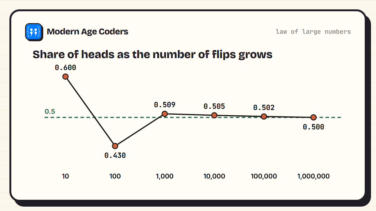
After 10 flips the share of heads was 0.60, and after 100 it was 0.43. By a million flips it was 0.4997. Small samples are noisy; large samples settle. This is why a survey of 20 people can be misleading, and why the average of a large sample is more trustworthy than a small one.
The gambler's fallacy
If a coin lands heads five times in a row, is tails "due"? It feels like it should be. But a coin has no memory: each flip is independent, so the next one is still 50/50. We flipped two million simulated coins and looked at every flip that came straight after five heads in a row:
import random

random.seed(11)
flips = [random.random() < 0.5 for _ in range(2_000_000)]

after_streak = [flips[i] for i in range(5, len(flips)) if all(flips[i - 5:i])]
print(f"times we saw 5 heads in a row: {len(after_streak):,}")
print(f"next flip was heads: {sum(after_streak) / len(after_streak):.3f}")times we saw 5 heads in a row: 63,063
next flip was heads: 0.504Out of 63,063 streaks of five heads, the next flip was heads 0.504 of the time, essentially a half. The law of large numbers does not work by "balancing out" past results; it works because a few early streaks get swamped by millions of later flips. Believing otherwise is called the gambler's fallacy, and it has cost gamblers a great deal of money.
Three rules that do most of the work
| Rule | When to use it | Example |
|---|---|---|
| AND: multiply | Both of two independent events happen | Two sixes on two dice: 1/6 × 1/6 = 1/36 |
| OR: add (then subtract any overlap) | Either of two events happens | A 1 or a 2 on one die: 1/6 + 1/6 = 2/6 |
| NOT: 1 minus | An event does not happen, or "at least one" questions | No six in one roll: 1 − 1/6 = 5/6 |
The last rule is the secret weapon for "at least one" questions. The probability of at least one six in several rolls is hard to count directly, because there are so many ways it could happen. But it is simply 1 minus the probability of no sixes at all, and that is easy: multiply 5/6 by itself once for each roll.
The question that started it all
In 1654 a French gambler, the Chevalier de Méré, brought questions about dice bets to the mathematician Blaise Pascal. Pascal's letters with Pierre de Fermat about such problems helped found probability theory. The bets were roughly these: is it good to bet on at least one six in 4 rolls of a die? And on at least one double six in 24 rolls of two dice? Both look like the same deal scaled up, since a double six is 6 times rarer and you get 6 times as many rolls.
import random

# Exact, using "at least one" = 1 - "none"
one_six_in_4 = 1 - (5 / 6) ** 4
double_six_in_24 = 1 - (35 / 36) ** 24
print(f"at least one six in 4 rolls:        exact {one_six_in_4:.4f}")
print(f"at least one double six in 24 rolls: exact {double_six_in_24:.4f}")

random.seed(1654)
trials = 200_000
a = sum(any(random.randint(1, 6) == 6 for _ in range(4)) for _ in range(trials))
b = sum(any(random.randint(1, 6) == 6 and random.randint(1, 6) == 6 for _ in range(24)) for _ in range(trials))
print(f"simulated over {trials:,} tries: {a / trials:.4f} and {b / trials:.4f}")at least one six in 4 rolls: exact 0.5177
at least one double six in 24 rolls: exact 0.4914
simulated over 200,000 tries: 0.5184 and 0.4907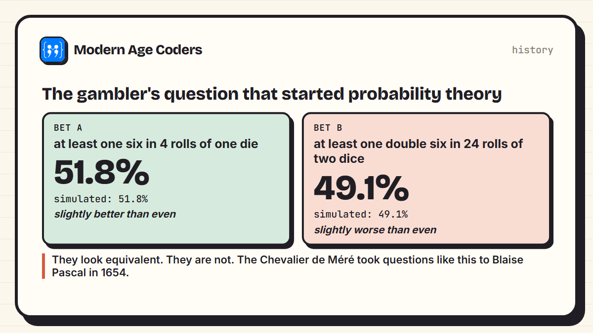
Bet A wins 51.8% of the time, a little better than even. Bet B wins only 49.1%, a little worse. The "1 minus none" rule gives both answers in one line each, and the simulation of 200,000 tries confirms them. The scaling argument failed because probabilities of "at least one" do not grow in proportion to the number of tries.
The Monty Hall problem
This puzzle comes from the American game show Let's Make a Deal, and it became famous in 1990 when a magazine columnist gave the correct answer and many readers, some of them mathematicians, wrote in to insist she was wrong. There are three doors: behind one is a car, behind the others are goats. You pick a door. The host, who knows where the car is, opens a different door to show a goat, and offers you the chance to switch. Should you?
import random

def play(switch):
    doors = [0, 1, 2]
    car = random.choice(doors)
    pick = random.choice(doors)
    # the host opens a door that is not your pick and does not hide the car
    opened = random.choice([d for d in doors if d != pick and d != car])
    if switch:
        pick = next(d for d in doors if d != pick and d != opened)
    return pick == car

random.seed(5)
games = 100_000
for switch in (False, True):
    wins = sum(play(switch) for _ in range(games))
print(f"{'switch' if switch else 'stick ':<6}: won {wins / games:.3f} of {games:,} games")stick : won 0.334 of 100,000 games
switch: won 0.667 of 100,000 games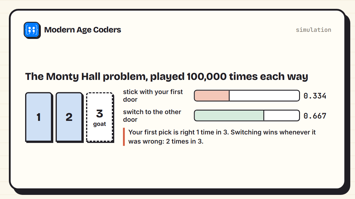
Sticking won 0.334 of the time and switching won 0.667. The reason: your first pick is right only 1 time in 3. The host's choice does not change that, because he always shows a goat whatever you picked. So in the 2 out of 3 games where your first pick was wrong, the remaining closed door must hide the car, and switching wins. If it still feels wrong, imagine 100 doors: you pick one, the host opens 98 goats, and one door stays shut. Would you switch now?
Why simulation is so useful here
When your intuition and a calculation disagree, a simulation settles it. Writing one also forces you to state the rules precisely, like the fact that the host never opens your door or the car's door. Many people get Monty Hall wrong because they never pin those rules down.
Where probability is used
- Weather forecasts: "70% chance of rain" is a probability based on many similar past situations.
- Medicine: how likely a positive test result is to be correct depends on how common the illness is, a question closely related to the false alarm problem with AI detectors.
- Games and sport: from board game strategy to deciding when to take a risk.
- Machine learning: many AI models output probabilities, not certainties, which is part of why they make mistakes.
When intuition and calculation disagree, run the experiment. Probability is one of the few areas of maths you can test a million times before lunch.
How we teach it
Probability fits the principles on our how we teach page well. We show the same problem three ways until the aha lands, and here that means counting, a formula and a simulation, which is exactly how this post checks each idea. Students explain their thinking, which matters in a topic where first guesses are so often wrong. Our live maths classes run one to one or in small groups of 5 to 10.
Frequently asked questions
Probability is how likely something is to happen, on a scale from 0 (impossible) to 1 (certain). When outcomes are equally likely, it is the number of outcomes you want divided by the total number of outcomes.
Count the outcomes that give the event you want, and divide by the total number of equally likely outcomes. For two independent events both happening, multiply their probabilities. For at least one of something, work out 1 minus the probability of none.
7. It can be made in 6 of the 36 equally likely ways, a probability of 1/6. Totals of 2 and 12 are the least likely, with 1 way each.
The mistaken belief that past random results change the next one, such as thinking tails is due after several heads. Each coin flip is independent. In our simulation, after five heads in a row the next flip was heads about half the time.
You should switch. Switching wins 2 out of 3 games because your first pick is only right 1 time in 3, and the host always reveals a goat. Our simulation of 100,000 games gave 0.667 for switching and 0.334 for sticking.
As you repeat a random experiment more times, the proportion of outcomes gets closer to the true probability. A few coin flips can give very uneven results, but a million flips give very close to half heads.
Children often meet simple probability words like likely and unlikely in primary school, and calculate probabilities as fractions in the early secondary years. Simulations in Scratch or Python make the ideas concrete at almost any age.