How Do Maps Find the Fastest Route? Dijkstra's Algorithm

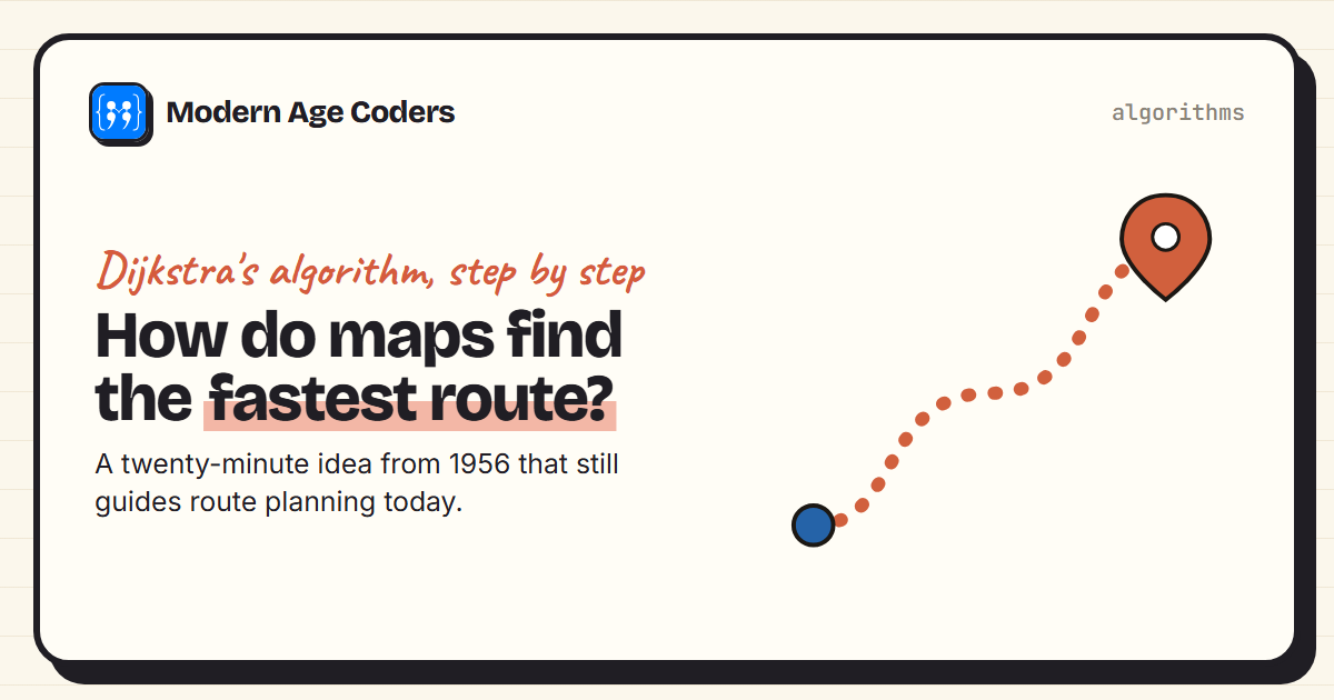
Ask a map app for directions and it picks the fastest route from millions of possible roads in a moment. The classic method behind route finding is Dijkstra's algorithm, and it is simple enough to follow by hand on a small map, and to write in about twenty lines of Python.

This guide runs Dijkstra's algorithm on a small town, step by step, then compares it with two tempting shortcuts that give the wrong answer. It ends with A*, the faster variant used in games and navigation, measured on a 10,000-place grid. Every result below comes from running the code.

The problem: a map is a graph

To a computer, a road map is a graph: places are nodes, roads are edges, and each edge has a weight, here the travel time in minutes. Finding the fastest route means finding the path between two nodes with the smallest total weight. Here is our town:

# A small town: travel times in minutes along each road (roads go both ways)
roads = [
    ("Home", "Shop", 2), ("Home", "Park", 4), ("Home", "Library", 13),
    ("Shop", "Park", 1), ("Shop", "Market", 3), ("Park", "Library", 5),
    ("Library", "Market", 4), ("Library", "School", 3), ("Market", "School", 2),
]
graph = {}
for a, b, minutes in roads:
    graph.setdefault(a, {})[b] = minutes
    graph.setdefault(b, {})[a] = minutes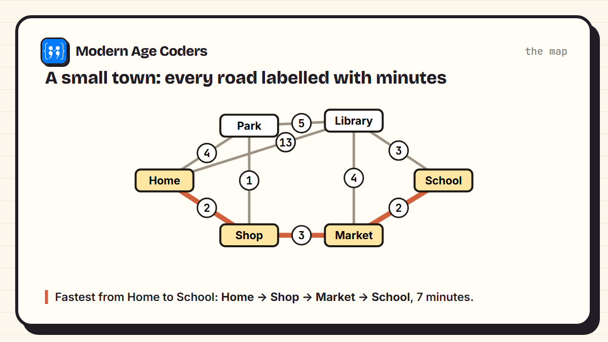

Dijkstra's algorithm, step by step

In 1956, the Dutch computer scientist Edsger Dijkstra wanted a problem that non-programmers could understand, to show off a new computer in Amsterdam. He later said he designed the shortest-path algorithm "in about twenty minutes", sitting on a café terrace, and it was published in 1959. The idea:

1. Give the start a time of 0 and every other place a time of infinity (not yet reached).
2. Pick the unsettled place with the smallest time and settle it: its time is now final.
3. For each road out of it, see if going that way reaches a neighbour faster than its current best time. If so, update it.
4. Repeat until the destination is settled.

The key insight is step 2. Because all travel times are positive, once a place is the closest unsettled one, no other route can ever reach it more quickly, so its time is final. In code, a priority queue (Python's heapq) hands back the closest place each time:

import heapq
from town import graph

def dijkstra(graph, start, goal):
    best = {start: 0}               # fastest known time to each place
    came_from = {}
    queue = [(0, start)]
    settled = []
    while queue:
        time, place = heapq.heappop(queue)     # always expand the closest unsettled place
        if place in settled:
            continue
        settled.append(place)
        if place == goal:
            break
        for nxt, minutes in graph[place].items():
            new_time = time + minutes
            if new_time < best.get(nxt, float("inf")):
                best[nxt] = new_time
                came_from[nxt] = place
                heapq.heappush(queue, (new_time, nxt))
    route = [goal]
    while route[-1] != start:
        route.append(came_from[route[-1]])
    return best[goal], route[::-1], settled

if __name__ == "__main__":
    minutes, route, settled = dijkstra(graph, "Home", "School")
    print("settled in this order:", " -> ".join(settled))
    print(f"fastest route: {' -> '.join(route)} ({minutes} minutes)")

settled in this order: Home -> Shop -> Park -> Market -> School
fastest route: Home -> Shop -> Market -> School (7 minutes)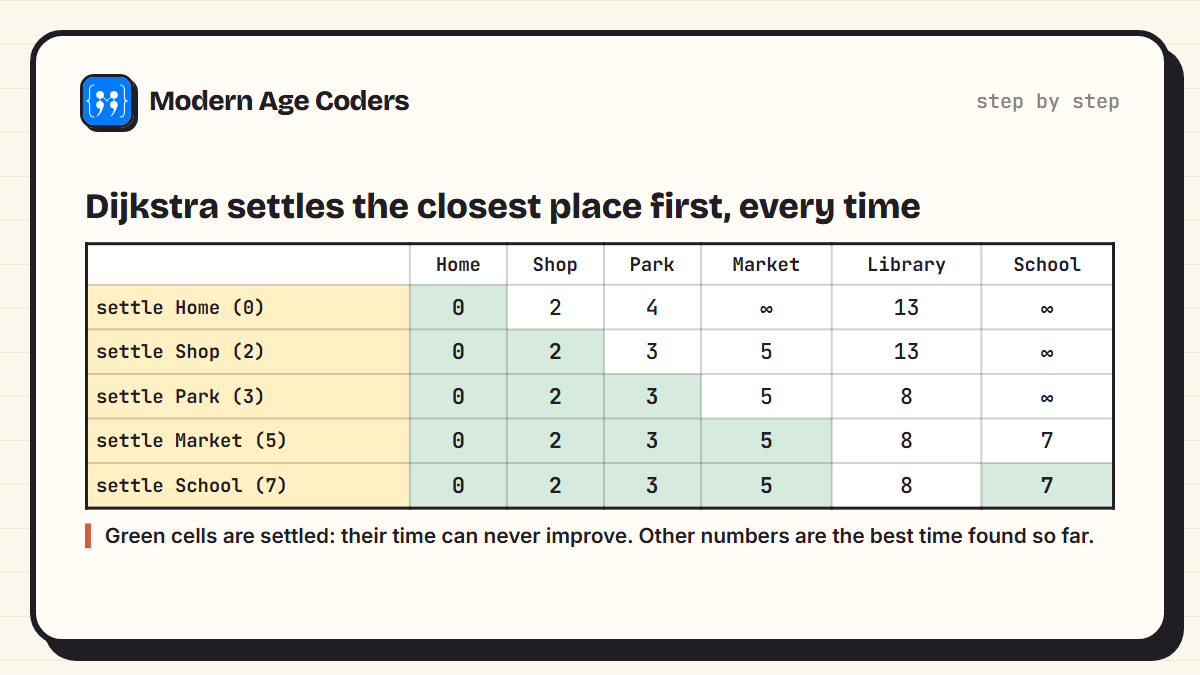

Dijkstra settled Home, Shop, Park, Market and then School, in order of distance from Home, and found Home -> Shop -> Market -> School in 7 minutes. Notice that it never settled the Library: by the time School was reached, the Library was known to be further away, so it was not needed.

Two tempting shortcuts, and why they fail

It is worth seeing why a smarter method is needed. The first shortcut: from wherever you are, take the quickest road you have not used yet. This is a greedy strategy:

from town import graph

# A tempting shortcut: always take the quickest road from where you are now
place, route, total = "Home", ["Home"], 0
while place != "School":
    options = {p: m for p, m in graph[place].items() if p not in route}
    place = min(options, key=options.get)
    total += options[place]
    route.append(place)
print(f"greedy route: {' -> '.join(route)} ({total} minutes)")

greedy route: Home -> Shop -> Park -> Library -> School (11 minutes)

The second: take the route with the fewest roads, which is what a breadth-first search finds when it ignores travel times:

from collections import deque
from town import graph

# Fewest roads (ignoring how long each one takes): breadth-first search
queue, seen = deque([["Home"]]), {"Home"}
while queue:
    path = queue.popleft()
    if path[-1] == "School":
        break
    for nxt in graph[path[-1]]:
        if nxt not in seen:
            seen.add(nxt)
            queue.append(path + [nxt])
minutes = sum(graph[a][b] for a, b in zip(path, path[1:]))
print(f"fewest roads: {' -> '.join(path)} ({len(path) - 1} roads, {minutes} minutes)")

fewest roads: Home -> Library -> School (2 roads, 16 minutes)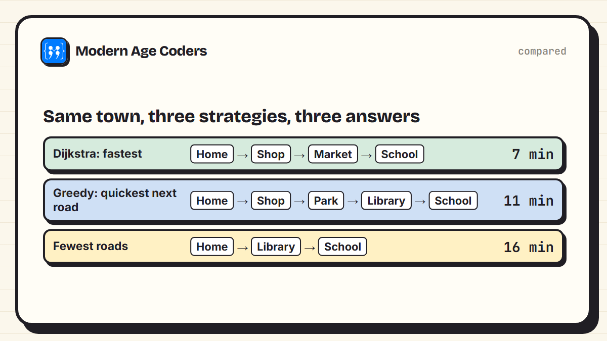

The greedy route took 11 minutes: the 1-minute road from the Shop to the Park looked attractive, but it led the wrong way. The fewest-roads route used only 2 roads but took 16 minutes, because one of them is a long 13-minute road. Dijkstra's 7 minutes beats both, because it compares every possibility in order of total time rather than trusting one step at a time.

A*: aiming at the goal

Dijkstra explores outwards evenly in every direction, like ripples in a pond, even away from where you are going. A* (pronounced A-star) adds an estimate of the time still to go, such as the straight-line or grid distance to the goal, and explores the places that look most promising first. As long as the estimate never overestimates, A* still finds the fastest route. We compared them on a 100 × 100 grid town:

import heapq, random

# A 100 x 100 grid of streets: most blocks take 1 minute, some busy ones take 4
N = 100
rng = random.Random(3)
cost = [[1 if rng.random() < 0.8 else 4 for _ in range(N)] for _ in range(N)]
start, goal = (50, 20), (50, 80)                # across the middle of town

def search(use_estimate):
    best, queue, settled = {start: 0}, [(0, 0, start)], set()
    while queue:
        _, time, (r, c) = heapq.heappop(queue)
        if (r, c) in settled:
            continue
        settled.add((r, c))
        if (r, c) == goal:
            return time, len(settled)
        for dr, dc in ((1, 0), (-1, 0), (0, 1), (0, -1)):
            nr, nc = r + dr, c + dc
            if 0 <= nr < N and 0 <= nc < N:
                t = time + cost[nr][nc]
                if t < best.get((nr, nc), float("inf")):
                    best[(nr, nc)] = t
                    # A*: add a lower bound on the time still to go (every step costs at least 1)
                    guess = (abs(goal[0] - nr) + abs(goal[1] - nc)) if use_estimate else 0
                    heapq.heappush(queue, (t + guess, t, (nr, nc)))

for name, flag in [("Dijkstra", False), ("A*", True)]:
    time, visited = search(flag)
    print(f"{name:<9} fastest time {time} minutes, places settled {visited:,} of {N * N:,}")

Dijkstra  fastest time 72 minutes, places settled 6,420 of 10,000
A*        fastest time 72 minutes, places settled 467 of 10,000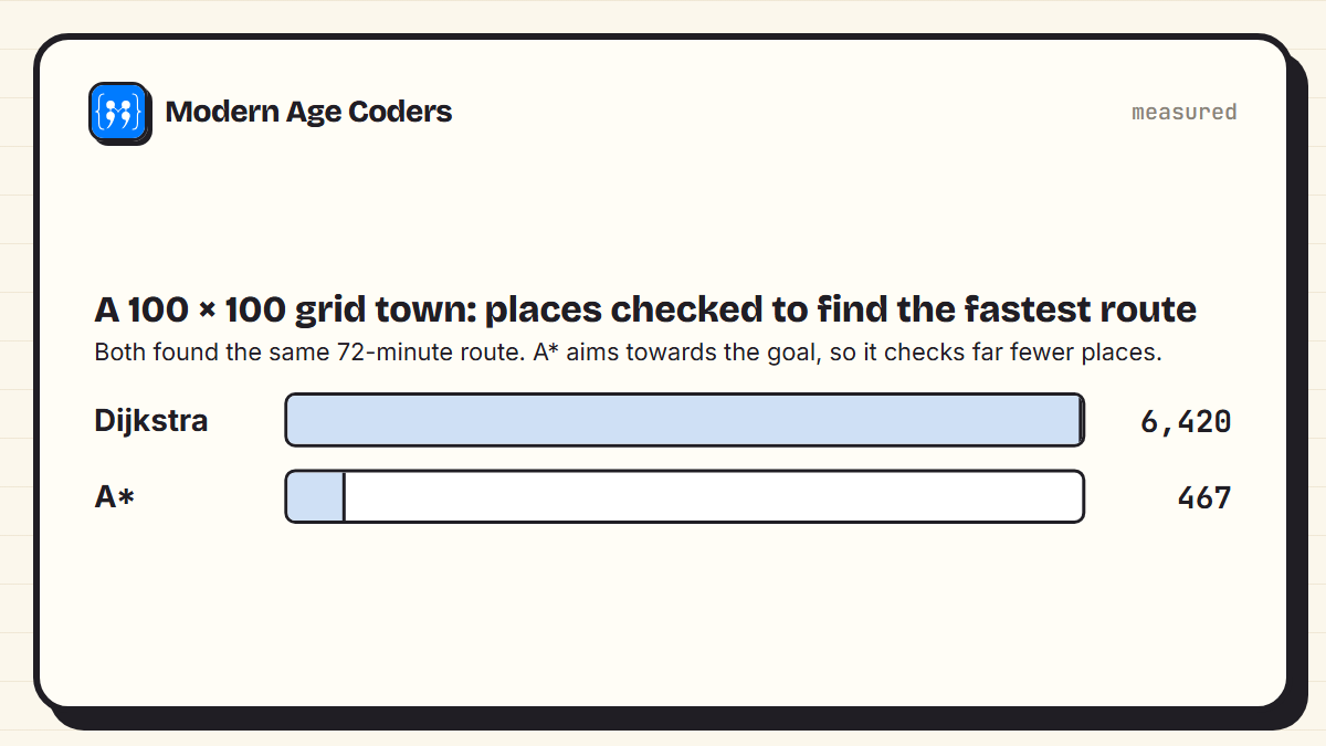

Both found the same 72-minute route, but A* settled 467 places while Dijkstra settled 6,420, about 14 times fewer. How much A* helps depends on how good the estimate is. When we first tried a grid where every street took 1 to 5 minutes at random, corner to corner, the estimate was weak and A* settled 9,994 places against Dijkstra's 10,000. Real navigation apps go further still, using live traffic data and precomputed shortcuts across the road network, but Dijkstra's idea is at the heart of it.

Where shortest paths are used

• Navigation apps for driving, walking and public transport.
• Games: characters finding their way round obstacles, usually with A*.
• The internet: routers choosing paths for data. A widely used routing protocol, OSPF, uses Dijkstra's algorithm.
• Deliveries and logistics: planning routes for vans and couriers.

Settle the closest place first, and never look back. That one rule finds the fastest route.

How we teach it

Dijkstra's algorithm suits a principle on our how we teach page: trace line by line until the student can predict every step. Filling in the settle table by hand on a small map, then checking it against the code, is exactly that. Seeing the same problem solved three ways, greedy, fewest roads and Dijkstra, makes clear why the algorithm works. Our data structures and algorithms course runs one to one or in small groups of 5 to 10.

Frequently asked questions