Table of Contents
Big O notation sounds like advanced maths, and most explanations make it look that way. It is actually one simple idea: as the amount of data grows, how much more work does your code have to do? A program that handles 100 items instantly might take a second with 100,000 items, or an hour, and Big O is the language programmers use to predict which.
This guide explains Big O without the heavy maths. Every claim is backed by code you can run: step counts measured by actually running the algorithms, and timings measured on a real machine. By the end you will be able to look at a loop and say what its Big O is, and know why it matters for exams, interviews and real programs.
What Big O actually measures
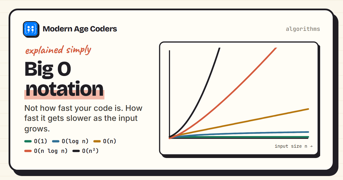
Big O does not tell you how many seconds a program takes. That depends on the computer, the language, and what else is running. Instead, it tells you the shape of the growth. If you double the input, does the work stay the same, double, or quadruple?
That is why it is written with n, the size of the input. O(n) reads as "order n" and means the work grows roughly in proportion to n. O(n²) means it grows with n times n. The O is just a label saying "we are describing the growth, not the exact count".
- O(1), constant. Looking up the first item in a list, or a value in a dictionary. The same work whether there are 10 items or 10 million.
- O(log n), logarithmic. Binary search in a sorted list. Each step throws away half of what is left, so a million items need only about 20 steps.
- O(n), linear. Checking every item once, like finding the largest number in an unsorted list.
- O(n log n). Good sorting algorithms, including the one Python's sorted() uses.
- O(n²), quadratic. Comparing every item with every other item. Fine for 100 items, painful for 100,000.
Watching the growth: steps counted by running the code
Here are three real algorithms, each with a counter that adds one for every basic step. The program runs them on lists of increasing size and prints the counts. Nothing here is estimated.
def linear_search(items, target):
    steps = 0
    for item in items:
        steps += 1
        if item == target:
            break
    return steps

def binary_search(items, target):
    steps, low, high = 0, 0, len(items) - 1
    while low <= high:
        steps += 1
        mid = (low + high) // 2
        if items[mid] == target:
            break
        if items[mid] < target:
            low = mid + 1
        else:
            high = mid - 1
    return steps

def compare_all_pairs(items):
    steps = 0
    for i in range(len(items)):
        for j in range(i + 1, len(items)):
            steps += 1
    return steps

print(f"{'n':>9} {'linear':>9} {'binary':>7} {'all pairs':>14}")
for n in (10, 100, 1_000, 10_000):
    data = list(range(n))
    worst = n - 1                      # the last item: the worst case for a linear search
print(f"{n:>9,} {linear_search(data, worst):>9,} {binary_search(data, worst):>7,} {compare_all_pairs(data):>14,}") n linear binary all pairs
10 10 4 45
100 100 7 4,950
1,000 1,000 10 499,500
10,000 10,000 14 49,995,000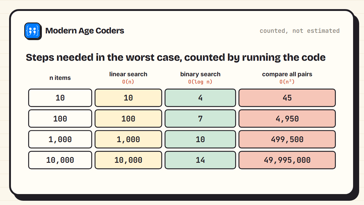
Read down each column. Every time n gets ten times bigger, linear search does ten times more work. Binary search adds only three or four steps. Comparing all pairs does about a hundred times more work, because ten times more items means ten times more items to compare, each against ten times more others. At 10,000 items that is nearly fifty million comparisons, for a list that fits comfortably in memory.
Why binary search is so fast
Binary search only works on sorted data. It looks at the middle item, decides which half the target must be in, and throws the other half away. Halving 10,000 repeatedly reaches 1 in about 14 steps, which is exactly what the counter shows. That halving is where every O(log n) comes from.
How to read Big O from code
You do not need to count steps every time. A few rules of thumb cover most code you will see in school, college and interviews.
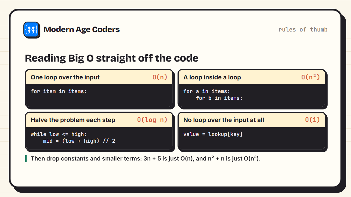
- Find the loops that depend on the input. A loop that runs once per item is O(n). A loop that always runs 10 times, whatever the input, is O(1).
- Nested loops multiply. A loop over n inside another loop over n is O(n × n) = O(n²). Three levels deep is O(n³).
- Loops one after another add. Two separate loops over the input are O(n + n) = O(2n), which is still O(n).
- Drop constants and smaller terms. Big O cares about what dominates when n is huge. 3n + 5 becomes O(n). n² + 100n becomes O(n²), because at large n the n² part swamps everything else.
- Watch for hidden loops.
x in my_listlooks like one step but is a loop inside Python. Put it inside your own loop and you have written O(n²) without noticing.
A real example: list or set?
That last rule causes more slow beginner programs than anything else, so it is worth seeing properly. Checking whether a value is in a Python list means looking at items one by one: O(n). Checking whether it is in a set uses a hash table to jump straight to where the value would be: O(1) on average. This program measures both, with the same data and the same thousand lookups:
import random
from time import perf_counter

random.seed(1)
for n in (10_000, 100_000, 1_000_000):
    numbers = list(range(n))
    as_set = set(numbers)
    lookups = [random.randrange(n) for _ in range(1_000)]

    start = perf_counter()
    for x in lookups:
        x in numbers              # a list checks items one by one: O(n)
    list_time = perf_counter() - start

    start = perf_counter()
    for x in lookups:
        x in as_set               # a set jumps straight to the item: O(1) on average
    set_time = perf_counter() - start

print(f"n = {n:>9,} list {list_time*1000:9.2f} ms set {set_time*1000:6.3f} ms")n = 10,000 list 67.94 ms set 0.536 ms
n = 100,000 list 1115.18 ms set 0.607 ms
n = 1,000,000 list 11211.89 ms set 3.188 ms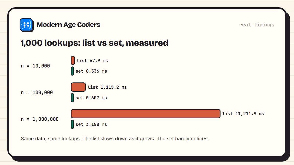
At a million items the list took about 11,212 milliseconds for a thousand lookups, and the set took about 3.2. Your exact numbers will differ, but the shape will not: the list's time grows with the size of the list, and the set's does not. That is exactly what O(n) versus O(1) predicts.
The same idea, fixing a slow program
A classic beginner task is checking whether a list contains any duplicate. The obvious solution compares every pair, which is O(n²). The better one remembers what it has already seen in a set, which is O(n). Both give the same answer:
import random
from time import perf_counter

def has_duplicate_slow(items):          # O(n^2): compare every pair
    for i in range(len(items)):
        for j in range(i + 1, len(items)):
            if items[i] == items[j]:
                return True
    return False

def has_duplicate_fast(items):          # O(n): remember what you have seen
    seen = set()
    for item in items:
        if item in seen:
            return True
        seen.add(item)
    return False

random.seed(2)
data = random.sample(range(10_000_000), 5_000)    # 5,000 different numbers, so no duplicate

start = perf_counter(); slow = has_duplicate_slow(data); t_slow = perf_counter() - start
start = perf_counter(); fast = has_duplicate_fast(data); t_fast = perf_counter() - start
print("same answer:", slow == fast)
print(f"compare every pair: {t_slow:.3f} s")
print(f"use a set:          {t_fast:.4f} s")
print(f"about {t_slow / t_fast:,.0f} times faster")same answer: True
compare every pair: 1.137 s
use a set: 0.0022 s
about 513 times fasterNothing clever happened. The fast version simply avoided doing the same work over and over. That is what most Big O improvements look like in practice: not a genius algorithm, but noticing that a loop inside a loop can become a lookup.
Big O of everyday Python operations
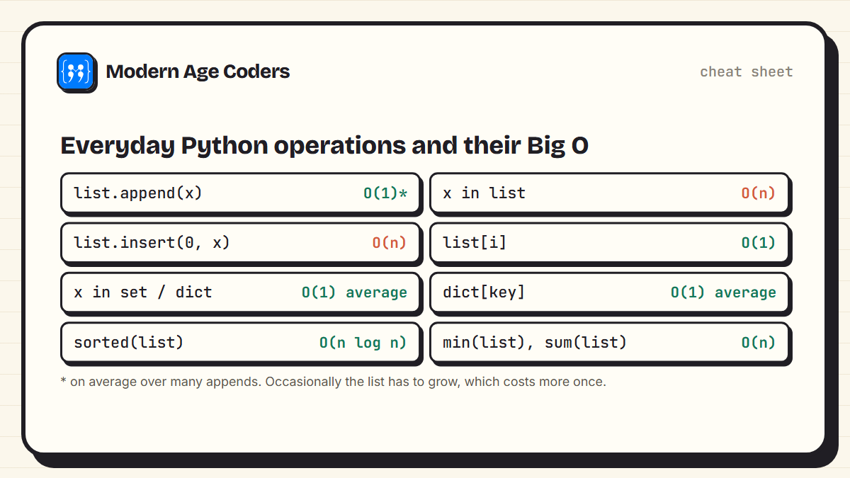
| Operation | Big O | Note |
|---|---|---|
| list.append(x) | O(1) on average | Occasionally the list resizes, but averaged over many appends it is constant |
| list[i] | O(1) | Jumping to a position is instant |
| x in list | O(n) | Checks items one by one |
| list.insert(0, x) | O(n) | Every other item has to shift along |
| x in set, dict[key] | O(1) on average | Hash tables jump straight to the right place |
| sorted(list) | O(n log n) | About as fast as a general sort can be |
| min(), max(), sum() | O(n) | Each has to look at every item once |
Best, worst and average case
You will sometimes see Big O described as the worst case. Linear search is O(n) because in the worst case the item is at the end, or missing, and every item gets checked. If the item happens to be first, it takes one step, but you cannot plan around luck. Interviewers and exam questions almost always mean the worst case unless they say otherwise.
Dictionaries and sets are the main place where the average case matters. Their lookups are O(1) on average, which is what you get in practice, though a deliberately badly-behaved input can make them slower. For everyday programming you can treat them as constant time.
Why it matters for exams, interviews and real code
- School and college exams. AP Computer Science, A level and university data structures courses all expect you to compare algorithms like linear and binary search, and bubble sort against merge sort, by their growth.
- Competitive programming. Contest problems are designed so the obvious O(n²) solution runs out of time. Our post on moving from USACO Bronze to Silver shows exactly this wall, measured.
- Technical interviews. After you solve a problem, the next question is almost always "what is the time complexity, and can you do better?"
- Real software. Code that works on your test file of 50 rows can fall over on a real file of 5 million. Knowing Big O is how you spot that before your users do.
Big O is not about making fast code faster. It is about not writing code that falls over when the data gets real.
How we teach it
Our data structures and algorithms course is taught live in Python, Java and C++, one to one or in small groups of 5 to 10. It follows the principles on our how we teach page, including tracing code line by line until a student can predict every step, which is the same skill that makes Big O intuitive rather than memorised.
Frequently asked questions
Big O notation describes how much more work an algorithm has to do as its input grows. O(n) means the work grows in proportion to the input, O(n squared) means it grows with the square of the input, and O(1) means it stays the same no matter how big the input gets.
O(n) means linear time: the work grows in direct proportion to the size of the input. If you double the number of items, the work roughly doubles. Looking at every item in a list once, such as finding the largest number, is O(n).
O(log n) means the work grows very slowly, because each step cuts the remaining problem in half. Binary search is the classic example: searching a sorted list of a million items takes only about 20 steps.
Not for every input size. O(1) means the time does not grow with the input, but that constant time could still be large. For big inputs, O(1) wins, which is why Big O focuses on growth rather than exact speed.
Look at the loops that depend on the input size. One loop over the input is O(n), a loop inside a loop is O(n squared), and repeatedly halving the problem is O(log n). Add loops that run one after another, multiply loops that are nested, then drop constants and smaller terms.
Because Big O describes what happens as the input becomes very large. At that scale, doing 3n steps instead of n steps matters far less than whether the work grows like n or like n squared. Constants depend on the computer and language, while the growth rate does not.
Yes. Almost every technical interview asks for the time complexity of your solution and whether it can be improved. Knowing the common patterns, such as replacing a nested loop with a set or dictionary lookup, is one of the most useful interview skills.